May 2020 Release Notes

The dystopia has worsened in Bangalore. Workers who live on daily wages are being forced to move back to their hometowns due to the lack of work and high cost of living. And even that wasn’t very straightforward because not all trains are running and India is a huge country. All this resulted in a kilometer long line at the Palace Grounds, strung together by humans and their luggages and littler humans fighting an invisible virus, the merciless heat and the weight in their hearts. And we’re just getting started.

While we’re on the topic of dystopia, William Shirer’s “The Rise and Fall of The Third Reich” is the most eye-opening piece of documentation on the Nazi regime that threatened to destroy our world, the book is closely followed by the HistoryTV documentary of the same name. With Adolf Hitler, Shirer asks us to appreciate his genius on his way to grabbing power but also wonder how much of everything he achieved can be attributed to luck. The more I read history, the more I’m tempted to believe that though we can extract certain patterns of human behaviour, we are never masters of our fate. I might disagree with Shakespeare’s Cassius in this regard, maybe we aren’t underlings and the fault is literally in our stars.

And speaking of stars, SpaceX was set to launch two NASA astronauts, Doug Hurley and Bob Behnken, from Cape Canaveral on NASA’s behalf, but the flight was scrubbed about 18 minutes before takeoff because of something none of us can control: the weather. It was an anticlimactic end to a day of anticipation, albeit a common enough occurrence for human spaceflight. They are going to try again early morning tomorrow, and I hope I get to watch a successful launch.

Simple Harmonic Motion

Let’s look at Simple Harmonic Motion. I remember how I was initially taught the concept. SHM is defined as any motion where

There are some functions that fit this very well but the most commonly known ones are sinusoidal functions. But it turns out that there’s a way to conclusively show that SHM’s will be sinusoidal in nature.

Consider a string fixed at one end of stiffness constant $k$, attached to a mass $m$ at the other end. Once in motion, the force $F$ by the string can be written as $F = -kx,$ which implies that $a = -\frac{k}{m}x.$ For our purposes, we shall assign $k/m = 1$ which would make $a = -x.$

Now, let us think of the position $x$ and the velocity $v$ of the mass at any given time. They would change by the following rule:

If we plot the position and velocity on a two-dimensional plane, it is easy to see that the change is actually a 90 degree rotation scaled up the small time-change. This is easier to see in the complex plane. More formally:

where $i = \sqrt{-1} = e^{i\frac{\pi}{2}}$. This means that, for every $z,$ we can write the change in state with respect to time as $\Delta z = -i \cdot z\Delta t.$ All this is very good, but where does it show the required periodicity? There is an intuitive aspect that we need to understand here, and that is the fact that all such changes will lie on a circle.

We can justify this in many ways, the most simple one is to understand that as $\Delta t \rightarrow 0,$ the locus of the points will trace out a circle. If it is so, we can write:

From this, it is easy to compare the real and imaginary parts of $z$ and get back the results we were taught in high school.

$e^x$ and the Poisson Distribution

Remember the exponentials section from last month? I have some additional material. As it turns out, we can obtain the Poisson distribution from the expansion of $e^x,$ let’s go!

We know the expansion of $e^x$

simplifying / rescaling / multiplying by $e^{-\lambda},$ we get:

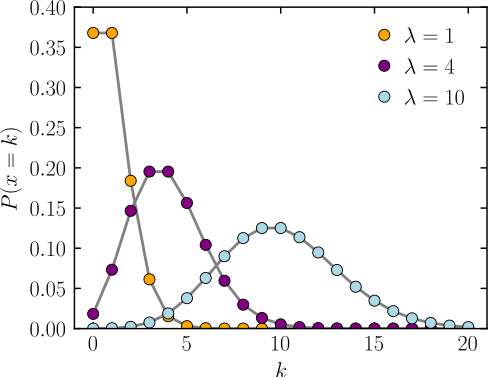
We now have a series that sums up to one, if you’ve been in a ProbStat class recently, you will know that we’re dealing with a distribution function. In this case, for the probability mass function, we just take a single step and evaluate. The Poisson distribution in all its glory is:

I want to look at the infinite sum in closer detail once again, let us write it out:

To get the $i^{th}$ step, we need to multiply the $(i - 1)^{th}$ step by $\lambda$ and divide it by $i.$ And when we scale the whole thing down, we get a nice distribution.

Natural Logarithms!!!

Question: Consider the numbers between 1,000,000,000,000 and 1,000,000,001,000. What is the proportion of these numbers that are prime?

A simple Python function will solve this problem for us:

import numpy as np
import math

def get_primes(n_min, n_max):
  result = []
  for x in range(max(n_min, 2), n_max):
    has_factor = False
    for p in range(2, int(np.sqrt(x)) + 1):
      if x % p == 0:
        has_factor = True
        break
    if not has_factor:
      result.append(x)
  return result

In [1]: get_primes(0, 50)
Out[1]: [2, 3, 5, 7, 11, 13, 17, 19, 23, 29, 31, 37, 41, 43, 47]

In [2]: get_primes(1000, 1050)
Out[2]: [1009, 1013, 1019, 1021, 1031, 1033, 1039, 1049]

We can see that the number of primes lessens as the arguments to get_primes() increase. This is all very obvious. Let’s now return the proportion and check for the values in our question.

import numpy as np
import math

def get_primes(n_min, n_max):
  result = []
  for x in range(max(n_min, 2), n_max):
    has_factor = False
    for p in range(2, int(np.sqrt(x)) + 1):
      if x % p == 0:
        has_factor = True
        break
    if not has_factor:
      result.append(x)
  return (n_max - n_min) / len(result)

In [1]: get_primes(10**12, 10**12 + 1000)
Out[1]: 27.027027027027028

Mathematicians know that the density of primes at any point on the number line is equal close to the natural log of that number. In this case, we can verify that math.log(10**12) = 27.6310211159.

With that bit of trivia out of the way, let us first recall that $y = \ln{x}$ is equivalent to $e^y=x.$ Why is this particular function called the natural logarithm though? Some more fun pieces of math coming up.

Consider the infinite series:

Now, we’ll manipulate this series such that we remove all non-primes, and scale down the powers of primes by the appropriate power they were initially raised to.

Another infinite series to play with:

Doing the same thing:

Another series with a known result:

We can actually figure out this result by generalizing it to:

Differentiating with respect to $x$ gives:

And to get the answer we require, we need to integrate this expression:

And the last one:

where $\gamma$ is a small constant. I hope that some will draw the connection to the integral of $\frac{1}{x}$ and try to answer why the sum turns out to be larger than the integral. I encourage the reader to write code or use a graphing calculator and check the other results out. The next question we should ask is why the derivative of $e^x$ always leads back to itself. One way we can come to this conclusion is by doing it the fundamental way. For $y = A^x:$

It would seem circular to put $A = e$ and finish the proof, so we can go back to the polynomial expansion of $exp(x)$ and differentiate that.

Local Memoization

• Fibonacci numbers:

$f(0)=0,$ $f(1)=1$ and $\forall n, f(n + 2) = f(n + 1) + f(n).$

def f(n):
    if n == 0:
        answer = 1
    elif n == 1:
        answer = 1
    else:
        answer = f(n-1) + f(n)
    return answer

n = int(input())
print(f(n))

The problem with this approach is that it is extremely time-consuming and we need a better option. The program is doing the same thing multiple times. Draw the recursion tree and check. So let’s add something to our code:

def f(n):
    print(f'f({n}) called')
    if n == 0:
        answer = 1
    elif n == 1:
        answer = 1
    else:
        answer = f(n-1) + f(n)
    return answer

n = int(input())
print(f(n))

Now if we try to find the 30th Fibonacci number, we see that f(1) was computed $832040$ times. Not optimal. Instead, let’s have a global dictionary and add a check before any compute.

memo = {}

def f(n):
    if n in memo:
        return memo[n]

    #print(f'f({n}) called')
    if n == 0:
        answer = 1
    elif n == 1:
        answer = 1
    else:
        answer = f(n-1) + f(n)

    memo[n] = answer
    return answer

n = int(input())
print(f(n))

Even for this, we don’t get the 1000th Fibonacci number Recursion Error: maximum recursion depth exceeded in comparison. We can add the following lines to the top of the code to increase the depth of the python stack

import sys
sys.setrecursionlimit(10**6)

But even this fails in case our OS’ internal stack for sufficiently large numbers: Segmentation fault (core dumped). Then we can actually do the same thing for our OS and find out the $100000^{th}$ Fibonacci number. The whole idea behind this discussion is to show that using memoization gives us massive time advantages.

Another not-so-trivial fact here is that as the numbers get huge, we cannot really stick to our old assumptions that additions and multiplications are constant operations. This is one of the first things we’re taught when we learn the Big-O notation. With big numbers, additions and multiplications require their own algorithms.

For Fibonacci numbers in particular, the time complexity depends on the number of digits of the $i^{th}$ Fibonacci number. More specifically, the number of digits in the $i^{th}$ Fibonacci number is linear in i. There is a class of problems similar to the one we tackled in which we can apply memoization to a similarly string effect.

Question: We’re given the size $n$ of an array $v$ and the values in that array: $v[0], v[1], \cdots ,$ Our task is to choose certain values such that we don’t pick values from adjacent slots. Find the strategy that maximizes the sum of values.

First approach: Good ol’ brute force. This is basically a combinatorial optimization problem, so one solution is to iterate over all possible solutions and keep a max variable. This is actually a good and preferable solution if the value of $n$ is around 20 or so.

Second approach: Recursive bactracking. Suppose we discard the $v[n - 1]$ slot, we have the same problem for the other $n-1$ slots. In this way, we make recursive calls. But if we do take the $v[n-1]$ slot, we cannot choose the $v[n-2]$ slot. So, the optimal solution in this case is the optimal solution for the first $n-2$ slots.

v = [int(_) for _ in input().split()]
N = len(v)

def solve(k):
    # question: what is the optimal solution for the first k slots?
    if k <= 0:
        answer = 0
    else:
        leave = solve(k - 1)
        take = solve(k - 2) + v[k - 1]
        answer = max(leave, take)

    return answer

print(solve(N))

What is the time complexity of this program? The time to process $n$ slots is the time to process one recursive call with $n - 1$ slots plus one with $n - 2$ slots. Similar to Fibonacci eh? The real value is more like $\Theta (n) = 1.6^n.$ So let’s apply a decorator and memoize this whole process.

import sys
sys.setrecursionlimit(10**6)
from functools import lru_cache

v = [int(_) for _ in input().split()]
N = len(v)

@lru_cache(maxsize = None)

def solve(k):
    # question: what is the optimal solution for the first k slots?
    if k <= 0:
        answer = 0
    else:
        leave = solve(k - 1)
        take = solve(k - 2) + v[k - 1]
        answer = max(leave, take)

    return answer

print(solve(N))

DIY: Iterative Solution, hint: use a dictionary?

Random Thoughts

Everything you ever wanted to know about negative numbers and weren’t afraid to ask!

MathProfessorQuotes

Medium posts are mostly trash but this article is really cool: Github Stars are overvalued

Basic git commands everyone should know about

Elon Musk on the Joe Rogan Podcast

Dr. Rhonda Patrick on the Joe Rogan Podcast

The Third Reich: Rise and Fall

Typesetting before $\LaTeX$

Terms of Service; Didn’t Read

ADAPT TO IMPACT: INSIDE THE HUMAN INTELLIGENCE OF PIETER ABBEEL

Diary of a Covid-19 Doctor: 14 Days in a NYC Hospital by WIRED

Building the Perfect Squirrel Proof Bird Feeder

The Past We Can Never Return To – The Anthropocene Reviewed

The Confessions of Marcus Hutchins, the Hacker Who Saved the Internet

Inside Italy’s COVID War by FRONTLINE

Yuval Noah Harari with India Today, the man never fails to amaze me with his powerful thought processes and articulate patterns of argument. Granted, the reporter is an idiot, but Prof. Harari still managed to get across his message.