Sums of random variables and convolutions

In probability theory, the probability distribution of the sum of two or more independent random variables is the convolution of their individual distributions¹. I learnt this while trying to make sense of the reparameterization trick in the diffusion forward process where we have to “add” two normal distributions.

This blog hopes to take the reader along my journey of understanding this idea. Even though — I hope I have presented it in an organized way — this blog is set out fairly sequentially so that there are no inane jumps, I did not actually go through it this way. When I first came upon the idea of adding two distributions, I skipped past it as being irrelevant. But I didn’t understand why the variances had to add up. So, I sat down to work it out only to realize I had no clue what adding two Gaussians meant. I did some Googling and found out that the product of two Gaussians was a Gaussian, and that this fact is used to prove that the convolution of two Gaussians is a Gaussian.

Now I had two more tasks in front of me. 1) Why is a convolution of two Gaussians a Gaussian? and 2) What does convolution have anything to do with adding the two distributions? I first solved the first question by solving the convolution integral, and then I watched a 3Blue1Brown video that helped me understand why you have to perform a convolution in order to add when you sample from two different distributions.

Finally, I went around trying to teach this to a few of my friends so they would ask me any questions I did not think about. This also helped me understand the whole thing in a much better way. Then I sat down to write this post.

A list of references if you want to work it out yourself:

• What are Diffusion Models by Lilian Weng — whose blog is one of the best things to read btw — where I was learning the diffusion theory from.
• Sum of Gaussian is Gaussian? which confused me because the accepted answer (with a dead link) says that it is not.
• Convolution of Gaussians is Gaussian which uses the FFT for the proof.
• The central limit theorem in terms of convolutions by Maxwell Peterson which finally cleared the fog blinding my eyes. “But this is the same thing as our convolution-of-distributions, because the density function of the sum of two random variables X, Y is the convolution of the density functions of X and Y.”

The Diffusion Forward Process

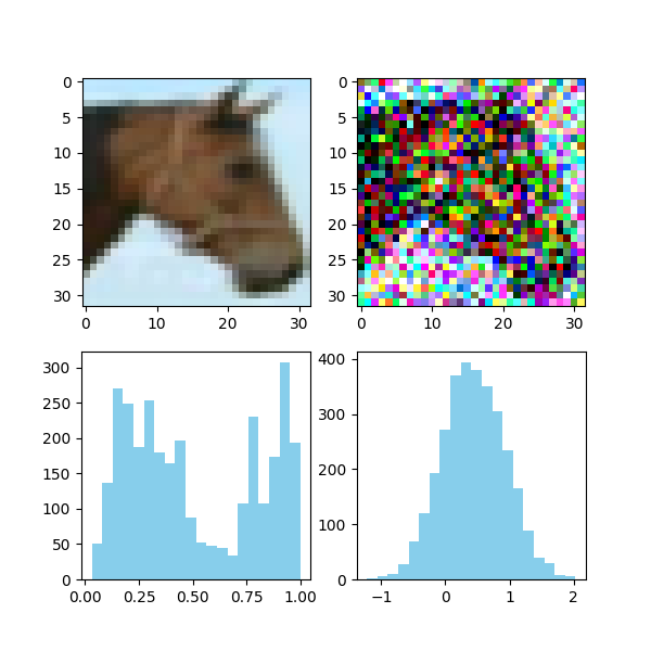
The diffusion forward process progressively adds Gaussian noise to a probability distribution (an image in this case) until the distribution very closely resembles a Gaussian distribution itself. The real data distribution $q(\mathbf{x})$ is transformed at each time step by the following rule

Figure 1. The diffusion forward process on an image from the CIFAR10 dataset.

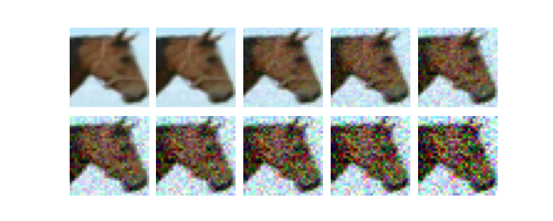
In practice, we compute this by multiplying the standard deviation to a normal distribution and adding a scaled mean to it ($\mathcal{N}(\mu, \sigma^{2})=\sigma\mathcal{N}(0, 1)+\mu$).

where $\mathbf{\epsilon}_{t-1}\sim\mathcal{N}(0, 1).$

Figure 2. The top two images show the first and final image, $\mathbf{x}_0$ and $\mathbf{x}_T$ respectively. The bottom two panels show the corresponding distributions of their pixel values. All three colour channels were flattened into one tensor before the histogram was produced.

In order to compute any $\mathbf{x}_t$ without having to go through all the previous time steps, we can substitute $\beta$ with $1-\alpha.$ Equation $(\tag(2)$ now becomes

where $\bar\alpha_t=\displaystyle\Pi_{i=1}^t\alpha_i.$ And finally,

Convolutions as sums of random variables

This is famously known as the reparameterization trick, and it was first used in variational auto-encoders. While I was reading through this math, I came to a stop between equations $(3)$ and $(4).$ I did not think it was immediately obvious that the sum of two normal distributions should be a normal distribution. In my head I pictured the bell curve of a gaussian and another bell curve of a different gaussian and attempted to add them only to realize I would get something like two peaks.

Figure 3. My first attempt at adding the probability distributions of two Gaussians.

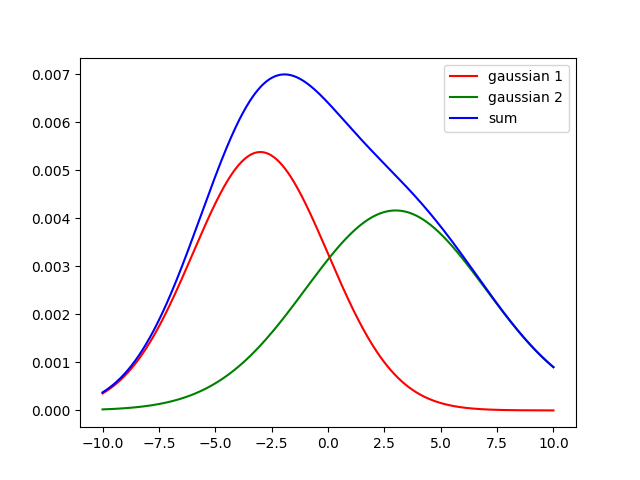
But this is obviously incorrect because this is adding the individual probabilies over the entire number line whereas what we need to do is compute the probability distribution of the random variable that arises when you sum the individual (and independent) normally distributed random variables. After a very long time, I found out that this could be achieved by performing a convolution between the individual probability distribution functions. The intuition really set in for me after I watched these two videos from 3Blue1Brown.

• Convolutions | Why X+Y in probability is a beautiful mess
• A pretty reason why Gaussian + Gaussian = Gaussian

We can see this in action using np.convolve. Just make sure that the “filter” has a smaller size, or the function will swap the two arrays around.

import numpy as np

array_a = np.array([0.1, 0.2, 0.3, 0.2, 0.2])
array_b = np.array([0.4, 0.3, 0.3])

convolved_array = np.convolve(array_a, array_b)

print(convolved_array)

>>> [0.04 0.11 0.21 0.23 0.23 0.12 0.06]

Convolution of two Gaussians

The last thing that remains is for us to verify that convolving one Gaussian with another gives a Gaussian as a result. We can check that by writing some code, and looking at the resulting curve, but it would be nice if we could rigorously prove it as well. Also, we have to verify that the variances add up (which is what is happening in the jump from equation $(3)$ to $(4)$).

A Gaussian probability distribution function is defined in the following way:

To make things easier for ourselves, and also to generalize, we can rewrite $g(x)$ as

which, if it has to be a Gaussian pdf, $A=\displaystyle\frac{1}{\sigma\sqrt{2\pi}},B=\displaystyle\frac{1}{2\sigma^2},$ and $C=\mu.$ We can perform a variable substitution $t=x-C$; which is the same as recentering the Gaussian. This doesn’t change the nature of the distribution.

Let us now take two functions $g_1(t)$ and $g_2(t)$

The convolution between them is defined as:

The trick to solving this integral is to convert it to the form $\displaystyle{\int_{-\infty}^{\infty}e^{-x^2}dx},$ which we know equals $\sqrt\pi.$ To do this, we complete the square inside the exponential.

Now the whole convolution becomes:

Now we know we have a Gaussian as the result of two Gaussians. The relationship between the variances can be gotten by substituting the value of $B=\frac{1}{2\sigma^2}$ everywhere:

$\blacksquare$

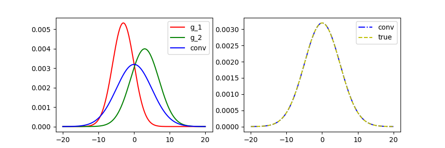
This is easier to do in code:

import numpy as np


def gauss(x, mu, sigma):
    G = (1 / (sigma * ((2 * np.pi) ** 0.5))) * np.exp(
        -0.5 * ((x - mu) ** 2) / (sigma**2)
    )
    return G / G.sum()


x = np.linspace(-20, 20, 1000)

N1 = gauss(x, -3, 3)
N2 = gauss(x, 3, 4)
N3 = gauss(x, 0, 5)  # -3 + 3 = 0; 5 = sqrt(3^2 + 4^2)

N1c2 = np.convolve(N1, N2, mode="same")

Figure 4. Convolution of two Gaussians on the left pane, and a comparison with the true Gaussian on the right pane.

Citation

Cited as:

Kilaru, Yasaswi Sri Chandra Gandhi. (April 2025). Sums of random variables and convolutions, New Ideas. https://kyscg.github.io/2025/04/23/diffusionconvolution/

Or

@article{kilaru2025diffusionconvolution,
  title   = "Sums of random variables and convolutions",
  author  = "Kilaru, Yasaswi Sri Chandra Gandhi",
  journal = "kyscg.github.io",
  year    = "2025",
  month   = "Apr",
  url     = "https://kyscg.github.io/2025/04/23/diffusionconvolution/"
}